Introduction

The Upthat manual describes the ‘front end’ of the tool, which has been designed to be used by practitioners, policy-makers and interested members of the public. This document reports the ‘back-end’ of the web application and the framework it uses to estimate modal shift at the city level. It is designed to be used by developers, researchers and data analysts. The aim is to show how the tool was built.¹

Scenarios

This section documents deliverable 2, scenario development, for the WHO Upthat project, which involves: (1) setting out high level policy scenarios of active transport uptake; (2) converting these changes into estimates of rates of shift towards walking and cycling down to route network levels; and (3) simulating the impacts of these scenarios on walking and cycling levels citywide. Scenario development will also be informed by the transport scenarios assessed in Accra and Kathmandu as part of UHI project activities.

High level priorities are to improve population health, air quality and safety levels. This means increasing the proportion of the population that gets regular physical activity, reducing motorized vehicle use in urban centers and providing walking and cycling routes that are away from or otherwise protected from motor traffic. Urban transport policies can meet each of these objectives, creating ‘win win win’ options. Reducing car use, for example, will directly improve air quality and indirectly improve health and safety levels.

Specific scenarios of change include:

‘Get walking’, referring to a global (meaning without spatial input components, but with spatially distributed consequences) walking uptake, as a result of citywide policies to promote safe and attractive walking.
‘Get cycling’, referring to a global scenario of cycling, as a result of citywide policies to provide safe cycleways.
‘Car diet’, a global, citywide scenario of multi-modal transport change, showing reduced levels of driving following disincentives to own and use cars.
‘Go public transport’, a global scenario of public transport uptake, linked to SDG 11.
‘Car free’, meaning investment in car free city centers, other car free spaces and other policies to reduce car ownership and use such as reductions in specific car parking spaces.

Citywide scenarios of change

To calculate scenarios of change, the minimum data requirements are the region’s current modal split and data that can be used as explanatory variables, including data on transport infrastructure and car parking spaces, and data on the provision of public transport options.

Mode split is one of the fundamental pieces of information that is known for most cities. For context, it’s useful to take a step back and consider the range of modal splits observed in a sample of cities worldwide. Many sources of mode share data are available, including the following (none of which were used due lack of access to the underlying data or other issues):

Transport Geography website, which provides an image of mode split
The TEMS mode split tool, which provides a map but not the underlying data
Various country-specific datasets

A problem with many datasets on mode split is that they ignore or oversimplify active transport (e.g. Aguil’era and Gr’ebert 2014). Examples of this are the OECD passenger transport dataset and the European Union’s Modal split of inland passenger transport, 2016 webpage, which omits walking and cycling:

This suggests the need for an open, international dataset on modal splits in major cities over time. To overcome these issues we searched for crowd-sourced data on mode split. The figure below shows the diversity in mode splits based on 108 (primarily wealthy) cities, based on data of the type shown in the table below from Wikipedia.

City	walking	cycling	pt	car	other	year
Detroit	1	0	2	92	5	2016
Amsterdam	4	40	29	27	0	2014
Bratislava	4	0	70	26	0	2004
Osaka	27	21	34	18	0	2000
Helsinki	37	10	30	22	1	2016

The figure shows that cars dominate the transport systems of most cities, accounting for a mode shares ranging from 18% (Osaka, Japan) to 85% (Adelaide, Australia). A more useful way to view travel systems from an active transport perspective is to view walking as the foundation of transport systems and all other modes to supplement walking (Tight et al. 2011). This view is shown on the right of the figure, which shows walking mode shares in the sample of cities ranging from only 3% to more than 1/3rd (in Madrid, Spain and Vilnius, Lithuania). It is interesting to note that while there is a roughly even distribution of mode shares by car, other modes have more skewed distributions. This could reflect the diversity of policies used to promote walking, cycling and public transport and the fact that cars tend to be the default. This implication is that if no policies have been implemented to promote alternatives, cars dominate.

The relationships between the different modes is illustrated in the figure below, which suggests competition between all modes and cars (with public transport seeming to be the biggest deterrent to driving in this dataset), and synergies between public transport and walking. This suggests that a reliable way to encourage walking in cities is through investment in public transport.

This city level data allows models of mode split to be developed, assuming there are sufficient explanatory variables defining the transport system.

Transport system data

Transport systems are complex, composed of hundreds of interrelated elements. For modelling purposes, it makes sense to condense available datasets down into a few key parameters per city, zone or origin-destination pair. The process of identifying and quantifying transport system variables should be be an open-ended and adaptable process that is able to respond when the input data changes (e.g. due to changes in the transport system or improved data availability/collection). The Global City Data dataset provides several transport-related variables on major cities, but the data are highly skewed towards wealthy cities, and are thus not suitable for developing nations. Instead, data from the Natural Earth open data repository was used for basic city statistics, including (the ones used in this project):

Population
Area (km²)
Elevation
Country

The city data, with these explanatory variables added, are shown in the figure below

A framework for estimating mode share needs to be flexible, to incorporate additional/modified variables that will become available. We suggest focussing on ‘scale free’, meaning that they do not depend on the city’s size. The scale free nature of such measures also means that they can be used to estimate mode shares not only at city levels but also at the level of ‘desire lines’ connecting origins and destinations, as with the use of average gradient as a predictor of cycling potential in the PCT (Lovelace et al. 2017). Some additional variables, such as distance and relative time/cost for alternative modes, only make sense when measured at the OD level.

Modelling mode shift

Treating mode share as a dependent variable involves multiple interrelated dependent variables, which is problematic for standard regression approaches. An alternative used in cycling potential research has been to ‘expand’ mode split data into individual categorical variables (Lovelace et al. 2017, supplementary information). This strategy is computationally intensive however.

The datasets presented in the previous section are examples of proportional outcomes, where we are interested in the mode split of all travel in a city. These types of data are common in ecological modelling (Douma and Weedon 2019), which provided a basis for investigating the question of citywide scenarios of mode shift in which modes are analogous to species. Dirichlet regression is a recently developed technique for modelling proportions based on a range of dependent variables (Maier 2014).

Building on this work, support for Dirichlet regression was added to the R package brms (Bürkner 2017), which implements a Bayesian modelling framework based on the stan C++ library, in 2018. The advantage of brms is that it estimates uncertainty, vital for effective ‘no-regrets’ policy making. A basic example of the outputs of a Dirichlet regression model run are shown in the figure below, which represents the result of a model run for a subset of 28 cities for which we have access to population (other explanatory variables included provision of metro and bikeshare schemes).

The result suggest that beyond a certain size, increasingly large city populations are associated with a lower proportion of trips made by driving in the sample of cities used. More explanatory variables can be added using this framework, including categorical variables such as has_metro, the results of which (that increase the mode share by public transport and notably walking in the results, which also show confidence intervals) are shown. Of course, the quality of the prediction relies on good input data predicting mode shift and relies on the assumption that cities are in equilibrium states. This strengthens the need for open data on mode shift at city, OD and local levels over time following a range of interventions.

Results using different explanatory variables on a slightly larger dataset (n = 101) show the generalize-ability of the modelling framework. The figure below shows more policy relevant explanatory variables: number of bus stops per inhabitant and the provision of a tram system, which is more viable in many cities than a metro system.

The figure above shows the marginal effect of changes to one variable, holding all other variables equal. The model accounts for fixed effects such as population density that are hard to change with policy interventions. The relationship between population density and mode split is interesting in itself however, as shown in the figure below.

Of course, we need more input data than the 101 cities taken from open data repositories shown above to reduce the confidence intervals. However, we have clearly demonstrated a robust and highly flexible way to model mode shift that accounts for the interrelations between different transport modes. The next step is to apply these models to real city datasets.

Estimates of rates of shift towards walking and cycling down to route network levels

Taking Accra as an example, let’s see how the modelling framework can estimate mode shift (remember this is based on a small input dataset and a proof of concept rather than final results).

# note: depends on data in the who3 repo
cities = readRDS("cities.Rds")
m = readRDS("model-result-brms-density-bus-stops-101.Rds")
class(m)
accra = cities %>% filter(City == "Accra") %>% 
  mutate(Density = Population / Area) %>% 
  select(Density, bus_stops_per_1000, has_tram, -geometry)

City	Density	bus_stops_per_1000	has_tram
Accra	4787.81	1.23008	FALSE

The current mode split can be estimated as follows:

mode_share_current_estimate = predict(m, accra)[, , ]

	walking	cycling	pt	car	other
Estimate	0.14	0.05	0.18	0.59	0.04
Est.Error	0.11	0.07	0.13	0.16	0.07
Q2.5	0.01	0.00	0.01	0.27	0.00
Q97.5	0.43	0.25	0.48	0.88	0.24

In the PT scenario, we can increase the provision of buses to 10 per 1000 people, representing a high level of provision within the range of the sample of cities worldwide:

Estimated change in mode share (percentage points)

	walking	cycling	pt	car	other
Central estimate	0.8	0.5	1.1	-1.9	-0.5

The result can be shown graphically, as shown in the figure below, that shows mode split estimates under the two model experiment conditions: one in which Accra has 1.2 bus stops per person (as it does currently) and one in which it has 3. The x axis shows that this model experiment can be generalized over the parameter space, in this case with x representing density, and the vertical line representing Accra’s density (~5000 people per km2):

Under this scenario, the central estimate of car use drops by 12 percentage points while the central estimates for walking and cycling grow, by 2 percentage points and 4 percentage points, respectively. This highlights the synergies between active transport modes and bus use implicit in the data, suggesting that a combination of strong investment in public transport and active transport infrastructure can be complimentary. As mentioned already, larger input datasets, in particular with more example datasets from Africa and the developing world in general in this context, are needed to reduce the large confidence intervals around these estimates.

The framework enables us to model changes in mode share that would result from changes in any variable, categorical or continuous. Based on the input data, the impact of a tram system in Accra could be simulated as follows:

As with any model, the usefulness of the outputs rely on the quality of the inputs and the assumptions underlying the model. These limitations, which reflect the paucity of open, curated data on mode shift in cities internationally, are covered in the next section. They are such that the current data (which only has one data point in Africa and only a handful of cities in the developing world) is not deemed of sufficient size and diversity to make useful predictions of modal shift. Instead of presenting results based on limited input data, the remainder of this section outlines how mode shift could be estimated, provided sufficiently large and diverse input dataset on mode shift following interventions. The basic tenets of this method are that:

Mode share in cities depends on measurable transport system characteristics such as number of bus stops, length of footways and walkways and cycleways and other explanatory variables.
A sufficiently large and diverse dataset on mode share and explanatory variables can be collected. In the examples presented here, the dependent variables are the more problematic data to access: we can get data on transport system characteristics by bulk download and analysis of large OSM datasets (although this is a time consuming and computationally intensive task).

Based on these tenets, an approach to estimate mode shift in response to the scenarios outlined above is detailed below. We have shown that we can model multi-modal responses to continuous and categorical variables in a robust Bayesian framework with explicit treatment of uncertainty. Under this framework, the scenario definition can be simplified to the identification and modification of explanatory variables that are available at the city level for a sufficiently large sample (500+) settlements with sufficient diversity to represent the changes that could take place in the cities under consideration.

Changes could be made in a systematic way to each of the predictors to represent change on the ground. Adding amounts to continuous variables by amounts determined by the input data, e.g. with 25^th, 50^th and 75^th percentile increases representing low, medium and high levels of change, with a modifier (e.g. \(1 - current_provision / max_provision\) ) to represent the law of diminishing returns, would be one way to achieve this (that was roughly the approach used in the example scenario of increasing bus stop provision in Accra).

To provide a concrete example, imagine that the maximum number of bus stops in the city dataset is 15 per 1000 people and that the 75^th percentile level of provision is 3 bus stops per 1000. In this case, an ambitious increase would be calculated for cities that currently have no bus stops, 1 bus stop, 10 and 15 bus stops per person as follows:

max_provision = 15
max_increase_in_provision = 3
current_provision = c(
  0,
  1,
  10,
  15
)
modifier = (1 - current_provision / max_provision)
increase_in_provision = max_increase_in_provision * modifier
future_provision = current_provision + increase_in_provision 
future_provision
#> [1]  3.0  3.8 11.0 15.0

For categorical variables, the changes are simpler: a one-size-fits-all change to a categorical variable that will only affect cities that do not currently have a specific piece of infrastructure (e.g. a tram system in the example above).

Get walking

This scenario refers to a global (meaning without spatial input components, but with spatially distributed consequences) walking uptake, as a result of citywide policies to promote safe and attractive walking.

Key variables that are readily available for most cities, that could be modified by policies, include (Kerr Jacqueline et al. 2016):

Provision of walking infrastructure, for example the percentage of the city’s transport network that is footway
Average distance of demand-weighted walking routes from major (and therefore likely polluted) roads
Measures of pedestrian safety, e.g. pedestrian fatalities per billion km (bkm) walked (where available)
Connectivity, which can be measured in terms of average circuity for walking trips

Get cycling

This scenario refers to a global scenario of cycling, as a result of citywide policies to provide safe cycleways.

The the provision of cycling infrastructure, which could be measured as km/person or as a percentage of the length of the total transport network
Number of cycle parking spaces per person
Number of cyclist fatalities per bkm cycled (where available)
The provision of free cycle training facilities
The provision of a cycle hire scheme

Other important variables include average gradient, type of cycle network, level or car ownership and directness of cycle routes compared with driving routes (Parkin, Wardman, and Page 2008).

Car diet

This scenario refers a global, citywide scenario of multi-modal transport change, showing reduced levels of driving following disincentives to own and use cars. Variables that could be modified in support of this scenario include:

The average number of lanes of traffic on roads in a city could be reduced, representing reduction of space on the roads for cars.
The distribution of speed limits in a city, for example represented by the proportion of roads on which the speed limit is above 30, 50 and 100 KM/hr. Real world data from crowd-sourced driving data, e.g. as provided by Uber, could enable the quality of these variables to grow over time
Speed limit enforcement, e.g. measured as number of prosecutions per bkm driven
Fuel tax

Go public transport

This scenario is a global scenario of public transport uptake, linked to SDG 11. It would involve modifying explanatory variables that represent public public transport provision. Variables we could change in this scenario could include:

Increase in the number of bus stops per person in the city, a crude measure which has already been demonstrated to be a powerful predictor of multi-mode shift away from cars. A specific scenario could increase the provision of bus stops by the median value in the data as outlined above.
Change in the percentage of the city’s area within walking distance (e.g. 300m) of public transport nodes such as bus stops and rail stations

Go car free

This scenario refers to investment in car free city centers and other spaces, other locally specific scenarios, such as reductions in car parking spaces.

The proportion of the transport network on which cars can travel
The provision of car parking spaces per person
Localized changes, for example making city centers car free, which could feed into the proportion of the network which is car free, weighted by travel levels into the zones which go car free

Other modifiable transport system variables

In addition to the specific scenarios outlined above, there are other important variables that could be modified in model experiments, either as stand-alone interventions, or to supplement specific scenarios. These include:

Percentage of the transport network that is dedicated to motor traffic (an alternative or supplementary measure could be the percentage of the city’s surface area dedicated to motor traffic)
Laws and other policies influencing new modes of transport such as electric bicycles and electric scooters.

Fixed effects

Many variables are outside the scope of policy intervention but are important to consider in models nonetheless. An example of a fixed effect in the example above was population density. However, the predictions of current mode split in Accra were unrealistic because other fixed effects were omitted. There was no variable accounting for the fact that in Accra most people cannot afford a car, for example. Also, differences in culture influence transport systems. Variables to account for these fixed effects could include:

Transport variables from the country that the city is in, e.g. % who drive overall
A measure of economic development, inequality-adjusted human development index (HDI) bands
Topographic and climate variables

Data limitations and discussion

The data requirements of a robust model to estimate mode shift in the Bayesian, multi-model framework outlined above are substantial. The preliminary results are inherently limited by the small size and skewed nature of the input city dataset, shown in the map.

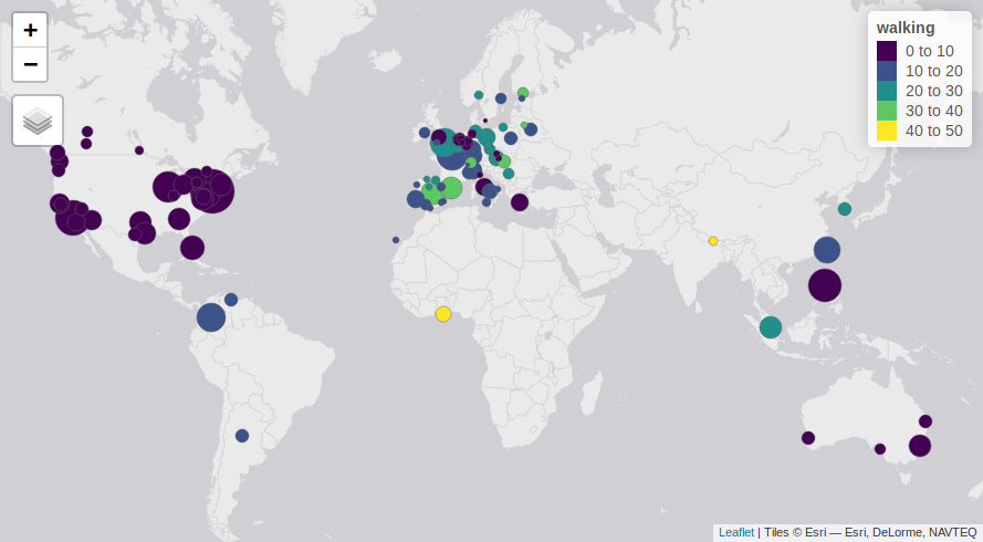
The map shows that there are only 2 cities with a high (40% +) level of walking, and these were cities that we added to the cities dataset. A priority for future is to expand this cities dataset to make it larger and more representative of cities where the Upthat tool is most likely to be used.

Scenario development accounting for the transport systems in Accra and Kathmandu, as part of UHI project activities, must be based on current transport data. An overview for Ghana (a proxy for the travel pattern in Accra) is shown below.

A more subtle data limitation surrounds modal categories. This is highlighted in the figure below which shows the full diversity of modes used in Accra from survey data on the left, and the effect of simplifying these categories into the modes which are most commonly reported. Future research should explore ways to gain data on and incorporate a richer diversity of transport modes.

A more conceptual question is how to account for the ordered nature of transport systems, e.g.:

Walking > Cycling > Public Transport > Cars

In terms of typical costs per km (assuming you have access to a bicycle) and the reverse order in terms of maximum speeds and energy costs per km. The framework outlined above could accept an arbitrary number of modes and mode size, speed and energy requirements could be accounted for by adding hybrid variables such as ‘maximum potential mode share by mode walking/cycling’ based on data on average trip distances per city (which may not be available for most cities) and distance decay parameters published in the literature.

Adapting the scenarios of change

The previous section outlines how additional of change can be added within the Bayesian framework using Dirichlet regression. The largest barrier to accurate predictions of mode shift following certain interventions, such as those described in the 5 scenarios above, was identified as being lack of data on mode split across cities, let alone with multiple time series enabling models to predict not only mode shift levels but change. This barrier is not insurmountable. If larger datasets on the dependent variable become available, the scenarios can be adapted to new city datasets as follows:

Acquisition of explanatory variables on transport systems. This can be done using bulk download and processing of OSM data, as has been demonstrated with the example of bus stops and tram systems above. Getting more explanatory variables for a larger sample size will take considerable time, perhaps 1 data scientist day per new variable added and 1 day per 200 cities.
Model training, assessment and prediction. This stage takes considerable time due to the computationally intensive nature of Markov chain Monte Carlo (MCMC) sampling used in Bayesian data analysis (McElreath 2016).
Estimates of uncertainty not only in the point estimates of mode split, but in the level of change that can be expected following specific interventions. For the confidence intervals displayed in the previous section to apply to the uptake of walking and cycling an extra stage is needed. This should not be difficult for a skilled Bayesian statistician but could take days for a data analyst new to the field of Bayesian statistics.
Refining the methods by which the top-down estimates of mode split feed into the flow generation model outlined in the calibration paper. In theory, the relationship between the top-down and bottom-up approaches should be two-way, because important information on a city’s transport system is ascertained in the process of routing across its transport network.

The bullet points above show that all of the technology and most of the data (although this is continuously evolving and depends on better mode split data across cities internationally) already exists for this approach to be deployed internationally and provides an indication of the amount of work required to do so.

Adapting the web app

The Upthat web app itself is fully reproducible. An up-to-date R installation on a modern computer should reproduce a fully working version of the app with the following commands:

remotes::install_github("atfutures/upthat")
upthat::runUpthat()

To modify the Upthat source code, download the repo and open it in an editor such as RStudio, e.g. with the following commands on a Linux terminal:

git clone git@github.com:atfutures/upthat
rstudio upthat/upthat.Rproj

To view the updated version of the app after making changes rebuild it, e.g. with Ctl+Shift+B in RStudio and then re-run the app with the command runUpthat(). For more on modifying shiny apps see the documentation associated with the package (Chang et al. 2015)or the in progress open source book Mastering Shiny (Wickham 2020).

Deploying upthat

To deploy a tool like Upthat so that it is publicly available as an interactive web app, the following resources are required:

A physical server with a reliable and fast internet connection or access to cloud compute resources
System administrator with web server experience to set-up Upthat on shiny-server
A skilled R developer to maintain packages and update Upthat with new data
A domain such as youcity.gov to provide a stable url to the app, e.g. www.yourcity.gov/upthat

References

Aguil’era, Anne, and Jean Gr’ebert. 2014. “Passenger Transport Mode Share in Cities: Exploration of Actual and Future Trends with a Worldwide Survey.” International Journal of Automotive Technology and Management 14 (3-4): 203–16. https://doi.org/10.1504/IJATM.2014.065290.

Bürkner, Paul-Christian. 2017. “Brms: An R Package for Bayesian Multilevel Models Using Stan.” Journal of Statistical Software 80 (1): 1–28. https://doi.org/10.18637/jss.v080.i01.

Chang, Winston, Joe Cheng, J J Allaire, Yihui Xie, and Jonathan McPherson. 2015. Shiny: Web Application Framework for R.

Douma, Jacob C., and James T. Weedon. 2019. “Analysing Continuous Proportions in Ecology and Evolution: A Practical Introduction to Beta and Dirichlet Regression.” Methods in Ecology and Evolution 10 (9): 1412–30. https://doi.org/10.1111/2041-210X.13234.

Kerr Jacqueline, Emond Jennifer A., Badland Hannah, Reis Rodrigo, Sarmiento Olga, Carlson Jordan, Sallis James F., et al. 2016. “Perceived Neighborhood Environmental Attributes Associated with Walking and Cycling for Transport Among Adult Residents of 17 Cities in 12 Countries: The IPEN Study.” Environmental Health Perspectives 124 (3): 290–98. https://doi.org/10.1289/ehp.1409466.

Lovelace, Robin, Anna Goodman, Rachel Aldred, Nikolai Berkoff, Ali Abbas, and James Woodcock. 2017. “The Propensity to Cycle Tool: An Open Source Online System for Sustainable Transport Planning.” Journal of Transport and Land Use 10 (1). https://doi.org/10.5198/jtlu.2016.862.

Maier, Marco J. 2014. “DirichletReg: Dirichlet Regression for Compositional Data in R.” 125. Department of Statistics and Mathematics, WU Vienna.

McElreath, Richard. 2016. Statistical Rethinking: A Bayesian Course with Examples in R and Stan. 1 edition. Boca Raton: Chapman and Hall/CRC.

Parkin, John, Mark Wardman, and Matthew Page. 2008. “Estimation of the Determinants of Bicycle Mode Share for the Journey to Work Using Census Data.” Transportation 35 (1): 93–109. https://doi.org/10.1007/s11116-007-9137-5.

Tight, Miles, Paul Timms, David Banister, Jemma Bowmaker, Jonathan Copas, Andy Day, David Drinkwater, et al. 2011. “Visions for a Walking and Cycling Focussed Urban Transport System.” Journal of Transport Geography 19 (6): 1580–9. https://doi.org/10.1016/j.jtrangeo.2011.03.011.

Wickham, Hadley. 2020. Mastering Shiny.

See the calibration report for details on the methods used to distribute trips across transport networks and estimating exposure to air pollution and physical activity.↩

Adaptation manual